似然比法在物证理化检验结果评估中的应用
[格若泽格兹•扎道若1, 2, *  , 安格妮孜卡•玛缇娜
1, 3 , 艾里克赞卓•米歇尔斯卡1 , 帕吹克•乌拉修克1, 3 ]
, 安格妮孜卡•玛缇娜|
|


新型犯罪日趋复杂,案件审判人员对高标准技术工作的需求不断增加,这些都要求研究新的证据评价方法,从而对各种微量物证理化检测数据的证据价值进行评估。证据评估方法能够反映法庭科学家在案件审理中的作用。这意味着上述数据(证据)应当在案件诉讼中控辩双方提出了相互对立的假设H1和H2的情况下接受评估,贝叶斯模型适用于这种情况下的证据评估。本文描述了在比较和分类(其实分类也是以比较为基础)问题中使用似然比方法(LR)对被观察的理化数据进行评估的原理。LR模型允许在一次计算中将所有重要的因素都包括在内,以此实现对相关理化数据的评估。这些因素包括,被比较样本间被比对理化数据的相似性,被测理化数据在有关总体中的稀有性,以及可能的误差来源(样本之内、之间的差异性)等。作为统计工具,LR模型只能用于仅以几个变量描述的数据库,而事实上大多数理化数据都是高度多维的(比如光谱),因此,需要使用缩维手段比如图形模型或适当的化学计量工具作降维处理,本文对此举例说明。需要指出,LR模型只应作为一种支持性(非决定性!)的工具,其结果(论)要接受严格的分析判断。换言之,统计方法并不能传达绝对的真相,采用的分析技术会有各自的不确定度,各种可能的错误答案也是统计方法的构成部分。因此,应当进行灵敏度检验亦即对所用分析方法作处理验证,从而确定其表现优劣。基于此,本文采用经验交叉熵方法举例说明如何对LR模型作校验。关于来源水平的理化数据评估,这涉及到比较样品是否源自于同一物体即是否具同一性的问题。通常,办案人员(法官、检察官或警察)会对被发现的取自于身体、衣服或鞋子的微量物证(显示与对照样本类似)是否发生了转移并留存下来的活动感兴趣,这就是所谓的活动水平检验,本文对此已有讨论分析。
The increasing complexity from new forms of crime and the need by those who administer justice for higher standards of scientific work require the development of new approaches for measuring the evidential value of physicochemical data obtained by application of numerous analytical methods during the analysis of various kinds of trace evidence. The methods used for evaluation of these data should reveal the role of the forensic experts in the administration of justice. This means that such data (evidence) should be evaluated in the context of two competing propositions H1 and H2 formulated by two opposite sides in the legal proceeding, i.e. prosecution and defence. Bayesian models have been proposed for the evaluation of evidence in such contexts. This paper describes the principle of likelihood ratio ( LR) approach for evaluation of physicochemical data in so-called comparison and classification (in fact, classification is also based on comparison) problems. The LR models allow including all of important factors in one calculation run where evidential value of physicochemical data is to evaluate. These factors are the similarity of observed physicochemical data in compared samples, the rarity of determined physicochemical data in relevant population, and the possible sources of errors (within- and inter-sample variability). The LR models, as statistical tools, can be only proposed for databases described by a few variables. However, most of physicochemical data are highly dimensional data (e.g. spectra). Therefore, it is necessary to apply methods of dimensionality reduction like graphical models or suitable chemometrics’ tools, with examples presented in the paper. The LR models should be always treated as a supportive (not the decisive!) tool and their results subjected to critical analysis. In other words, the statistical methods do not deliver the absolute truth as the levels of possible false answers are an integral part of these methods, in the same way like uncertainty related to the applied analytical techniques. Therefore, sensitivity convergence, an equivalent of the validation process for analytical methods, should be conducted in order to determine their performance. Thus, how to validate LR models is addressed in this paper by the example of application of Empirical Cross Entropy approach. There is the so-called source-level evaluation for physicochemical data as it helps to answer the question whether the compared samples are originated from the same object. Usually, the fact finders (judge, prosecutor, or police) are interested in recognizing the activity that made transferred and persisted of the recovered microtraces (which reveal similarity to control sample) from body, clothes or shoes. This is the so-called activity-level analysis, also discussed in the paper.
The application of numerous analytical methods to test evidence samples returns various kinds of data, i.e. morphological data (e.g. the number and thicknesses of layers in a cross-section of car paint), qualitative data (e.g. pigments present in a car paint sample), and quantitative data (e.g. concentration of elements in a glass fragment). The forensic scientists may be asked to comment on various competing statements (propositions) about the evidence (e.g. data obtained during analysis of microtraces), each of which may be true or false. They may refer to the immediate source of the evidence (e.g. is the piece of microtrace a glass sample?), an activity that has taken place (e.g. did the suspect break the window?), or an offence that has been committed (e.g. did the suspect steal something from the house?). These different types of propositions are known respectively as the source level, activity level and offence level propositions [1, 2]. Generally, a forensic scientist must consider two competing propositions relating to the evidence, one put forward by the prosecution (H1) and the other by the defence (H2) in a criminal case [1]. In such a situation, the aim of the forensic scientists is to evaluate the strength of support given by evidence data (E; such as elemental content of glass sample) to each of these two competing propositions so that the conditional probabilities Pr(E|H1) and Pr(E|H2), if possible in numerical way, is to estimate. Therefore, the best way to express this strength towards both propositions is to apply likelihood ratio (LR) test [3-5].
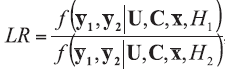
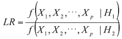
The law of likelihood (Eq. {1}) [6] tells that: if H1 implies that the probability that a random variable X takes the value x is Pr(X=x|H1) while hypothesis H2 indicates that the probability is Pr(X=x|H2), then the observation at X=x is the evidence supporting H1 over H2 if and only if Pr(X=x|H1) > Pr(X=x|H2), and the likelihood ratio measures the strength of that evidence:
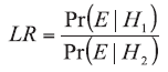
The likelihood ratio is not a probability, but a ratio of probabilities with values between zero (0) and infinity (∞ ). Usually the physicochemical data are of continuous type and therefore the probabilities are replaced by probability density functions f(E|H1) and f(E|H2). The decision rules are that H1 is supported at values of LR above 1 and H2 is supported at values of LR below 1. A value of LR close to 1 provides little support for either of the propositions, while the value, equal to 1, supports neither of hypotheses. Also, the larger (lower) value of the LR, the stronger (weaker) support of E for H1 (H2).
In order to make LR values more readable for fact finder, Evett, et al [2] proposed verbal equivalents of the calculated LR values:
· for 1 < LR ≤ 10, there is limited support for H1,
· for 10 < LR ≤ 100, moderate support,
· for 100 < LR ≤ 1000, moderately strong support,
· for 1000 < LR ≤ 10 000, strong support,
· for LR > 10 000, very strong support.
The likelihood ratio approach is a part of the Bayes’ theorem, expressed as:
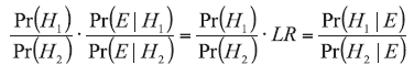
Pr(H1) and Pr(H2) are called prior probabilities and their quotient is called the prior odds. Their estimation lies within the competence of the fact finders (judge, prosecutor, or police) expressing their opinion about the considered hypotheses before the evidence is analyzed without having any further information in this matter. This opinion may be modified by the accounted LR values supporting one of the propositions and delivered by an expert after the analysis of evidence. It is the duty of a fact finder (police, or court), to determine which of the hypotheses is supported by the data and make decision, as mentioned previously, based on the results expressed in the form of conditional probabilities - Pr(H1|E) and Pr(H2|E), namely posterior probabilities, whose quotient is called the posterior odds [3, 4, 5].
When an evidence interpretation is investigated on a source level, then one of the problems solved by experts on the basis of obtained data is identification/classification problem, e.g., in glass cases, it is related to questions- whether the microtrace material found in debris is a glass object (H1) or not (H2), and if yes then does the glass fragment originate from container (H1) or float glass (H2)? The other forensic problem which could be solved at source level on the basis of obtained data is a comparison problem. This task is related to the question whether two samples, recovered (e.g. traces recovered from the suspect) and control (e.g. samples collected on the scene of crime), have possibly originated from the same object (H1) or from two different objects (H2). LR approach has become more popular in the evaluation of physicochemical data, e.g.:
a) elemental composition of glass samples determined by inductively coupled plasma mass spectrometry [7],
b) elemental composition of glass samples determined by scanning electron microscopy coupled with an energy dispersive X-ray detector [5, 8, 9, 10, 11, 12, 13, 14],
c) refractive index of glass fragments [15, 16],
d) lead isotopic ratios of glass determined by isotope ratio mass spectroscopy [17],
e) Semtex samples analysed by carbon and nitrogen isotope-ratio measurements [18],
f) car paint samples analysed by pyrolytical gas chromatography [19],
g) car paint samples analysed by Raman spectroscopy [20, 21],
h) car paint samples analysed by infrared and Raman spectroscopy [21],
i) fire debris analysed by gas chromatography [22],
j) colour of blue inks [23] or fibres determined by microspectrophotometry [10],
k) inks analysed by high performance thin layer chromatography [24],
l) ecstasy tablets [25],
m) determination of the geographical origin of olive oil [26] or wine [27].
Short introduction to models, which could be used for solving comparison and classification problems, is presented respectively in sections 2.1.1 and 2.1.2.
2.1.1 LR Models for Comparison Problem
When similarities are found between compared samples, the evaluation process should investigate whether they may be observed by chance. Thus, it is required the knowledge about the rarity of the measured physicochemical properties in a population (the relevant population, e.g., the population of car windows in the case of a hit-and-run accident) representative for the analysed casework, and the between-object variability. For instance, one would expect elemental composition from different locations of the same glass object to be very similar. However, equally similar elemental composition values could also be observed for different glass items. Therefore, information about the rarity of the determined elemental composition has to be taken into account. The value of the evidence is greater in support for the proposition that the recovered glass fragment(s) and the control sample have a common origin when the determined values are similar but rare in the relevant population, than when the physicochemical values are both equally similar and common in the same population [3, 5]. The information about the rarity of the physicochemical data could be obtained from the relevant databases available in the forensic laboratories.
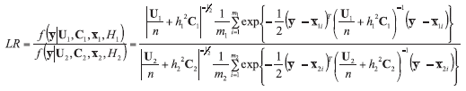
The idea of how to calculate an LR with inclusion of the rarity information is explained in the following example. Fragments of blue car paint (recovered sample) were found on the scene of a hit-and-run accident, in which a pedestrian died. A car that probably hit the pedestrian was found during the investigation. A sample of blue car paint was collected as a control material. An analysis with application of microspectrophotometry in UV range allowed to conclude that both samples had the same colour. This information (match of colours) is a piece of evidence (E), which can be evaluated in the context of two hypotheses:
H1 - recovered and control samples of blue car paint originate from the same blue car,
H2 - recovered and control samples of blue car paint originate from different blue cars.
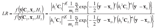
If H1 is true, the match is found between the control and recovered samples. In such circumstances, this event is a certain event, i.e. Pr(E|H1) equals to 1. Then it assumes that the blue car hit the pedestrian and a piece of this car’ s paint was transferred to the scene of the accident, being persisted there and recovered. In this case, the recovered and control samples of blue car paint originate from the same blue car in terms of the source level considerations. If H2 hypothesis is true, then the observed similarity of colour between recovered and control samples would be found by chance. It could happen, of course, as the same blue paint is used for painting many cars (also originating from different manufactures). Then, for calculating Pr(E|H2), the information on rarity of this colour of cars in the relevant population should be considered. For example, if the suspected car was bought in Europe in 2010, then it could be concluded on the basis of the available data (Table 1) that blue cars constitute 9% of all cars sold in Europe. This means that Pr(E|H2) could be assumed as 0.09, thus LR could be estimated on the following way: 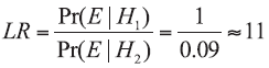
| Table 1 The frequency of particular colour of cars sold in Europe and China in 2010 (http://autokult.pl/2010/12/13/najczesciej-wybierane-kolory-lakierow-w-2010) |
This result means that an observed match between the recovered and control samples of blue car paint tends to be likely 11 times more supporting hypothesis H1 that recovered and control samples of blue car paint originate from the same blue car, than H2 hypothesis that recovered and control samples of blue car paint are from different blue cars. Moreover, an analysis of results presented in Table 1 allows to conclude that the higher support for H1 is observed when recovered and control samples originate from green or yellow/gold paint (LR=100), i.e. the most rarely occurring car paint. At the same time, the weakest support is obtained when these samples originate from black car (LR=4), i.e. the most commonly occurring car paint. It should be also highlighted that evidence value for particular data depends on the database selected. When the case circumstances are changed, e.g., that the accident happened in China, then according to information from Table 1, Pr(E|H2) could be assumed as 0.02. In such a situation, LR is estimated in the following way: 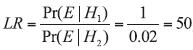
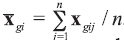
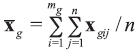
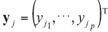
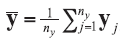
A background database is available with n measurements of p characteristics on each of m objects, so that data are in the form of p-vectors 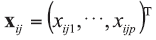
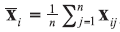

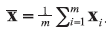
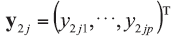


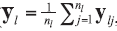
where 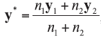


In the case of univariate data (p=1), all data vectors and matrices become scalars. Other LR models and examples of their application could be found in the literature [5, 7, 20].
2.1.2 LR Models for Classification Problem
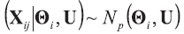
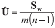
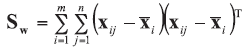
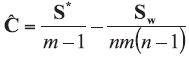
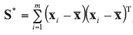
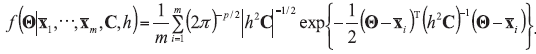
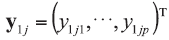
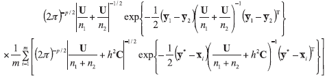
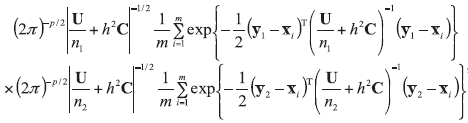
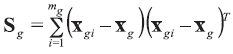
The following LR model should be taken into account in the case of assuming propositions on a source level but appropriately for classification problem. Consider there is a class g (g=1, 2) of mg of glass objects present in it. Each one is described by p variables and each is measured n times on a continuous scale within each object. Denote the object index as i so that 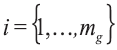


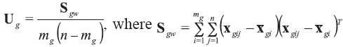
The between-object variance matrix Cg is estimated as: 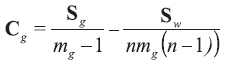
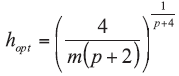
where hg, the smoothing parameter, 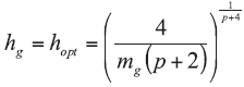
Other models and examples of their application could be found in Wł asiuk et al [26] and Zadora et al [5].
A limitation of multivariate modelling arises from the lack of background data from which to estimate the the assumed distributions of parameters such as means, variances, and covariances. For example, if objects are described by p variables, then it is necessary to reliably estimate the p means, p variances, and p∙ (p - 1)/2 covariances in the multivariate LR model:
This means that if an object is for example described by seven variables then it is necessary to reliably estimate seven means, seven variances, and 21 covariances in the full LR model, which is difficult to meet, when the background database contains a relatively small number of samples, e.g. 200 glass objects used in Aitken et al [8]. Thus, this process requires far more data than are usually available in typical forensic databases. This effect has been dubbed as the curse of dimensionality. This problem could be solved by making an assumption that the considered variables are independent, i.e. the problem with p variables could be then considered as a combination of p univariate problems. This is generally a naï ve approach as the variables are correlated in most of the analyzed problems: 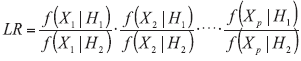
It was shown that the elements of the scaled inverse correlation matrix are the negative partial correlation coefficients [31], and that values of partial correlation (see Table 1 in Aitken et al [8]) can be used to construct a decomposable graphical model, converting the full probability density into cliques representing the product of several probability density functions in lower dimensions. The construction of graphical models can be illustrated for glass samples. The relationships between the elements in glass are not causal, and so the graphs are undirected. The graphical model has been selected by the sequential addition of edges after inspection of the partial correlation matrix. At first, the largest magnitude of partial correlation is chosen, and an edge is added between the two mostly correlated nodes. This process repeats until all nodes are part of the graphical model. A subset of variables, in which all the nodes are connected to each other, is known as a complete subgraph, and the corresponding subset of variables is known as a clique Ci. The intersections of elements between these two adjacent cliques in the graph (see Fig. 1 in Aitken et al. [8]) become separators Si. The factorisation of the p-dimensional density is given by: 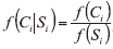
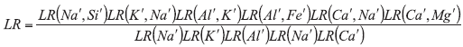
where LR(Na`, Si`) is the value of the likelihood ratio for multivariate densities with two variables (Na` and Si`) calculated by application of the LR model based on Eq. {3} and {4}; and similarly for LR(K`, Na`), LR(Al`, K`) and thus on. In the cases of bivariate problems, distribution parameters (two means, two variances and one covariance) could be estimated from a relatively small database, such as the 200-sample glass database. The graphical model approach was also satisfactorily used for the comparison of 36 car-paint samples described by seven variables derived from pyrolytic gas chromatography mass spectrometry. Similarly to glass example, the seven-dimensional problem was factorised into sets of bivariate and univariate problems [19].
Till now, the LR models have been applied for evidence evaluation only in situations when the number of objects in the database (m) exceeded the number of the variables (p) describing them (m > > p) [e.g. 5, 7, 8, 9, 11, 12, 13, 14, 18, 30]. The problem emerges in the case of highly multivariate data such as spectra stored in the numerical form, for which the situation is opposite (m < < p). In this case, it is indispensable to use huge database to reliably estimate the relevant parameters of the population for multidimensional data using statistical methods (e.g. LR approach). Such databases should consist of m objects, which number is far greater than the number of parameters (p) by which they are described. Moreover, for example when working with spectra databases, most of the parameters (e.g. absorbance or Raman scattering intensity measured by particular wave numbers) are highly redundant, i.e. the information they contain can be summarised in the form of much less variables than the original. Then the obvious solution to this problem may be reducing the number of the relevant parameters (variables) that are not indispensable for sufficient description of the characteristics for the limited number of the analysed samples. Moreover, such a procedure is also less computationally demanding than when working with all originally measured variables.
It is widely known that chemometric methods, such as principal component analysis (PCA), enable the most efficient data compression without losing too much information [32, 33]. It is therefore a natural way to use them for data dimensionality reduction. However, most of them are not accountable for many aspects, which are required from the forensic perspective (e.g. the rarity information). This is in turn addressed in the statistical methods, including LR approach. Therefore, it becomes natural to combine the advantage of the chemometrics’ abilities to reduce data dimensionality with the LR models meeting the requirements of forensic evidence evaluation.
One of the advantages of PCA is removing the variables’ mutual dependency and delivering new orthogonal variables. This feature could be used for LR model’ s construction on consideration of all principal components (PCs) based at the assumption that all information about the evidence may be relevant and should be taken into account in the forensic practice. Such a model involves the multiplication of LR values obtained for univariate problems, each of which built on single principal component i 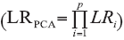
In research published by Martyna et al [20], LR models supported by wavelet transform and variance analysis were proposed for solving the comparison problem of polypropylene and blue car paint samples described by FTIR and Raman spectra, respectively. The results prove that the variables, generated after the wavelet transform, preserve various signal characteristics of sparse representation for the original signal by keeping its shape and relevant chemical information. The extracted variables sufficiently describe the analysed samples and carry the information suitable for solving the comparison problem using appropriate LR models.
An LR model, based on the results of linear discriminant analysis (LDA), was also proposed by Wł asiuk et al [26]. According to the LDA theoretical foundations, each sample’ s discriminant score corresponds to the posterior probability in the category described by H1 hypothesis (Pr(H1|E)) or category described by H2 hypothesis (Pr(H2|E)) and the decision is based on the comparison of values of such probabilities. These conditional probabilities, for practical reasons, are assumed to follow a parametric distribution, e.g. multivariate normal distribution, and that all categories have the same (pooled) covariance matrix. Posterior probabilities are computed on consideration of the information about prior probabilities (Pr(H1) and Pr(H2)) which are usually assumed as being either equal or proportional to category sizes. Therefore, having prior odds Pr(H1)/Pr(H2), the set of the LR values can be obtained through the posterior odds information acquired from linear discriminant analysis (Eq. {2}): 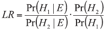
Another way of dealing with huge data dimensionalities is an approach presented by Zerzucha and Walczak [38], where the classical feature representation of samples characteristics can be replaced by what is called distance/score/dissimilarity representation. In this approach, each sample is described by its similarity expressed by distance measure (e.g. Manhattan, Euclidean) to the reference sample(s). This enables massive reduction of both data dimensionality and extracting features that are not easily observed in the classical feature representation. It is also worth noting that in LR models based on distance representation (so-called score-based LR models), the information about the rarity of the features is rather difficult to account for. This is why these models should be interpreted with great caution.
In previous points, it was presented that results of interpretation of physicochemical analysis of various types of forensic evidence can be enhanced using statistical methods. Nevertheless, such methods should be always treated as a supportive tool and their results should be subjected to critical examination. In other words, the statistical methods do not deliver the absolute truth as the levels of possible false answers are an integral part of these methods, in the same way like uncertainty related to the applied analytical techniques. Therefore, sensitivity convergence, an equivalent of the validation process for analytical methods, should be conducted in order to determine their performance.
False positive and false negative error rates in the case of a comparison problem or rates of incorrect classifications are common measures for evaluating decisions in forensic science [5, 39]. In an LR context, when a comparison problem is involved, a false negative error occurs when LR < 1 for a true-H1 comparison, and a false positive error occurs when LR > 1 for a true-H2 comparison. The term false negative refers to the fact that true-H1 likelihood ratio values should be greater than 1 but they are less than 1, they are falsely supporting the wrong proposition, H2. Conversely, true-H2 likelihood ratio values should be less than 1 yet they are greater than 1, they are falsely supporting H1; this is a false positive. In the case of solving a classification problem, rates of false classifications should be evaluated, i.e. a number of incorrect classifications into particular class (e.g. LR should be greater than 1 for a true-H1 class and an incorrect classification error occurs when LR > 1 for a true-H2class).
The rates of correct and incorrect LR model answers (false positives and false negatives, or incorrect classification rates) are limited measures of performance. They only provide information about supported proposition according to the threshold set at LR=1, but they ignore the strength of the support carried by the magnitude of theLR value. For instance, an LR value would be much worse if its value of LR=1000 than that of LR=2 in the case of true-H2 hypothesis. On consideration of only false positive, false negative and incorrect classifications rates, these two LR values are treated equally and no distinction between their strength is made. Generally, for everyLR model it is crucial that it delivers strong support for the correct hypothesis (i.e. LR > > 1 when H1 is correct and LR < < 1 when H2 is correct). Additionally, it is desired that if an incorrect hypothesis is supported by LR value (i.e. LR < 1 for true-H1 and LR > 1 for true-H2), then the LR value should concentrate close to 1, delivering only weak misleading evidence. Roughly speaking, according to Eq. {2}, it seems to be of great importance to obtain LR values that do not provide misleading information for fact finder. This implies that assessing the performance of the applied methodology for data evaluation requires the application of the Empirical CrossEntropy (ECE) approach [5, 40, 41, 42, 43]. Based on information theory, ECE considers the correctness of decisions made when assessing the statistic, e.g. LR model, performance. It is a method based upon the system of rewarding and penalising the experimental LR values. The penalty is assigned to the LR models’ responses that support the incorrect hypothesis, which is expressed by logarithmic strictly-proper scoring rules [5, 42, 46]. The higher of the support for the incorrect hypothesis, the greater penalty the model’ s response is assigned to:
a) if H1 is true: -log(Pr(H1|E)),
b) if H2 is true: -log(Pr(H2|E)).
The overall penalty rate (LS) is the weighted average of all values of penalties assigned to the LR models’ responses considered under the H1 and H2 hypotheses:
a) for a comparison problem, 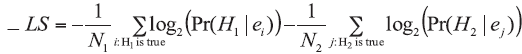
b) for a classification problem, 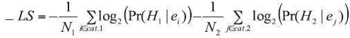
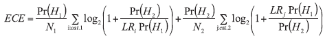
The ECE is then a modification of LS weighted by the relevant prior probabilities Pr(H1) and Pr(H2), and according to Eq. {2}, the LR model can be evaluated on the basis of the following expression:
a) for comparison problem:
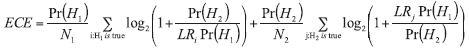
b) for classification problem:
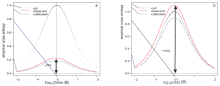
Even though the knowledge about prior probabilities can be acquired from a number of various sources, for example witnesses, additional evidences or police investigations, it is rarely directly available for forensic experts. Because of the fact that ECE can be computed only if the prior probabilities are known, ECE can be calculated for a set of all possible prior probability quotients (prior odds). In the so-called ECE plot (Fig. 1), three components can be distinguished:
a) observed curve (solid red) - represents the ECE values which are calculated in accordance with Eq. {5} or {6} for LR values subjected to the evaluation;
b) calibrated curve (dashed blue) - corresponds to the ECE values which are calculated for the LR values being transformed with the use of a pool adjacent violators (PAV) algorithm [5, 41, 44, 45]. This approach allows for the analysis of the unaltered classification or discrimination power of the LR values’ set. The calibrated curve serves as an indicator of the LR values with the best performance out of all other LR sets offering the same classification or discrimination power;
c) null or reference curve (dotted black) - refers to the situation where no value is assigned to the evidence. Always being the same, the null curve should be treated as a reference curve which represents the performance of a method always delivering LR = 1.
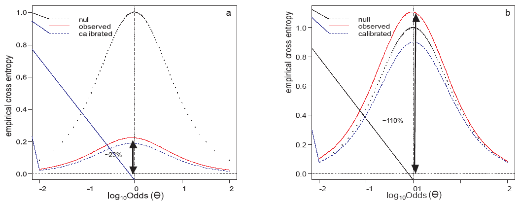 | Fig.1 Empirical cross entropy (ECE) plots for LR models with (a) satisfactory and (b) poor performance |
The interpretation of the relative location of the ECE curve for the experimental set of LR values (solid, red line) in relation to the remaining two (dashed and dotted lines) illustrates the performance of the method of evidence evaluation. If the LR values of the evidence evaluation are misleading to the fact finder, then the ECE will grow, and more information will be needed in order to know the true values of the hypotheses (Fig. 1). In other words, the higher the curve (e.g. obtained at the point of log10Odds(Θ )=0), the more uncertainty remains and therefore the worse the method of choice is for the interpretation of the evidence under analysis. If the curve appears to have greater values than the ones in the neutral method (Fig. 1b), the evidence evaluation introduces more misleading information than when no of the evidence evaluation exists at all.
It should be pointed out that fact finders usually are interested in recognising the activity that made transferred and persisted of the recovered mictrotraces (which reveal similarity to control sample) from body, clothes or shoes [3, 48]. This involves the question, for instance, whether the person who wore clothes on which glass microtraces were found broke the window of the car from which a GPS was stolen (H1) or not (H2).
It is an analysis about so-called the one of activity level. A difference between analysis on source and activity levels could be explained by the following example. The car was broken into by its window being broken. A sample of glass from the broken window was collected (control sample) and the suspect was arrested after several hours. Trousers and a jacket of the suspect were collected for analysis. Eight glass fragments which revealed similarity of elemental composition to the control glass sample were found during analysis of debris from clothes. In such a situation, a fact finder would like to know which of the two hypotheses is more supported by this evidence:
H1 - suspect broke the window,
H2 - suspect did not break the window.
In the aim to answer this problem, other factors than only those included in the evaluation on a source level (rarity determined in compared glass fragments’ elemental composition by SEM-EDX, within- and between-object variability) should be taken into account [48, 49], i.e.:
a) primary transfer - a probability of an event of transferring a particular number of glass fragment(s) revealing similarity to the control sample, their persistence and recovering after a specified time e.g. from clothes,
b) coincidental similarity of glass fragments found by chance - the probability of finding glass fragments similar to the control material but collected from a person neither having contacted with the suspect nor being on the scene of crime,
c) secondary transfer - the probability of an event of transferring the glass fragment(s) revealing similarity to the control sample from person A’ s clothes or from an object (e.g. chair) to the person B’ s clothes as a result of the direct contact.
In general, there could be lack of suitable databases which allow to make reliable estimation of these probabilities in most of cases. A solution is to apply LR models based on Bayesian networks (BNs) for the interpretation of problems related to an activity level [3, 47, 48, 50 - 53].
In this paper, a concept of LR approach for interpretation of physicochemical data for forensic purposes was described. If it was still not convincing that a forensic scientist must consider two competing propositions, then maybe the following example (not related to physicochemical data) could change it.
Blood stains were disclosed in the region of a shirt sleeve’ s cuffs of a person suspected of a murder. The suspect’ s version was that he was administering first aid to the victim, who had been stabbed with a knife, so that the bloodstains were visible on the shirt sleeves. If an expert issues an opinion in the context of only H2 (the version of the accused/defence), the conclusion could be that the version of the event that the bloodstains in the region of the shirt sleeve’ s cuffs arose in the course of administering first aid to the victim is probable. A conclusion formulated in this way may be considered as evidence by the fact finders (e.g. judge, prosecutor, defence) that this is what actually happened. However, in practice, it is difficult to estimate the probability of this event. Likely, for example, after the case files being read, this argument is established that the accused person took part in a fight and probably used a knife to stab according to the testimony of witnesses, thus the disclosed stains on the sleeves could have occurred in the described places due to the stabbing. In such an opinion held with an expert (H1), this version of the event is also probable. In other words, if - instead of the defence counsel - the prosecutor asks the question whether these stains could have arisen in a situation where the accused had been stabbing the victim with a knife, then, inquiring an expert opinion only in the context of one hypothesis (H1), the forensic expert could have written that the version of the event that bloodstains in the region of the shirt sleeve’ s cuffs arose in the course of stabbing the victim with a knife is probable. A conclusion formulated in such a way may be considered as evidence by the fact finder that the event actually happened that way. However, if assessing the evidence in the context of two hypotheses, and accepting that the formation of the bloodstains on the sleeves in the case of both conditions is equally probable, a statement should be that evidence in the form of disclosing bloodstains in the region of the shirt sleeve’ s cuffs supports each of these hypotheses to the same degree. This evidence is of little significance for the justice system, but it has been fairly assessed, i.e., it does not mislead the fact finders, and is more reliable than in the case of defining its value in the context of only one of the hypotheses.
One reason for the slow implementation of the LR models is that there is a very limited number of software that enables the calculation of the LR relatively more easier by those of the less experienced in programming (like most forensic experts). One example could be the calcuLatoR software for the computation of likelihood ratios for univariate data [54]. Therefore, in order to use these methods, case-specific routines have to be written using an appropriate software package, such as the R software [55], a “ comparison” package in R or R routines published in books [5, 39].
The authors have declared that no competing interests exist.
| [1] |
|
| [2] |
|
| [3] |
|
| [4] |
|
| [5] |
|
| [6] |
|
| [7] |
|
| [8] |
|
| [9] |
|
| [10] |
|
| [11] |
|
| [12] |
|
| [13] |
|
| [14] |
|
| [15] |
|
| [16] |
|
| [17] |
|
| [18] |
|
| [19] |
|
| [20] |
|
| [21] |
|
| [22] |
|
| [23] |
|
| [24] |
|
| [25] |
|
| [26] |
|
| [27] |
|
| [28] |
|
| [29] |
|
| [30] |
|
| [31] |
|
| [32] |
|
| [33] |
|
| [34] |
|
| [35] |
|
| [36] |
|
| [37] |
|
| [38] |
|
| [39] |
|
| [40] |
|
| [41] |
|
| [42] |
|
| [43] |
|
| [44] |
|
| [45] |
|
| [46] |
|
| [47] |
|
| [48] |
|
| [49] |
|
| [50] |
|
| [51] |
|
| [52] |
|
| [53] |
|
| [54] |
|
| [55] |
|